Chapter 21.2 - Data Assimilation, Sampling & Kalman Filtering

0:08 >> I want to continue talking about data simulation and common filtering and also issues of sampling that we have to consider when we think about using this common framework for data simulation. So, I want to talk first about the measurements and sampling. In the last part of our talk, the last section of our talk, what we did was we talked about the fact that I could actually make an observation of the system. You know, there's a full state space. But in practice, that never happens.

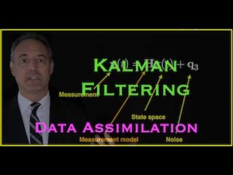
0:38 For instance, in weather, you can only make point observations at limited locations. And it could be that you have quite a few locations, but they're still limited when we typically think of our model as being sort of a continuous field. So, the idea behind this to say I have an observation which is actually a subset of the state space. So, H is my measurement model. So, I'm going to take H could be simply a mask of locations to measure. So, like I can only measure certain locations of X. So, H tells me it's those locations.

1:12 That's where I take a measurement. And Q3, of course, is going to be our noise term. So, we don't get a perfect measurement. So, the way this works, right, is I have a measurement of the system. And that measurement of the system is only in certain locations, okay, typically. So, that's my measurement model H. And here's my state space. I'm measuring a small section of the state space, and there's of course noise there. So, for instance, for instance, consider an airplane wing.

1:39 And if I had several measurements on the airplane wing, let's say five measurements of the airplane wing, but I'm trying to understand the whole flow physics, well, the H would be the five measurement locations. In other words, block everything out at these five locations, I get a measurement, and I have a noisy measurement there, but I'm trying to use those five locations to do a better job in making a prediction. In other words, assimilating it with what I have.

2:03 So, we have to take into account this reality that there's always going to be a a measurement matrix H in almost every system that we measure. In other words, we only have partial observations of the full state of the system. And partial observability is a common thing that we would have throughout engineering and science overall. Okay? So, we this common filtering framework accounts for that. So, let's start off with a 1D common filter, and let's focus only on the model error. So, what I mean by that is here's the true physics, let's say.

2:36 I'm going to the next state space, and I've written this as a discrete time dynamical system. So, I'm looking at time K + 1, and I get there from the model f of x of K. So, this is my dynamics model, and I hit x of K, I get to the future, and of course I have error there in the model itself. But, my model itself is perfect. So, the future state is what I am now plus f.

3:02 So, essentially I can get error here by not knowing x naught, but in this here it also tells me that yeah, but in addition to that, you also have the model error, which is going to be modeled by that Q of Q Q K + 1. So, what I'm going to do is take this and subtract from here. So, I'm going to take the left side here, subtract here, right side here, subtract from there. And what we have here then is this equation here, where now I'm going to expand this term in a Taylor series expansion around f of x naught.

3:37 And when I do that, expectation, so first term is f of x naught, which cancels this term, and then I get my derivative terms, second derivative terms. I just expand this out in a Taylor expansion, and I can rewrite this by squaring it into the following form. So, what I'm looking at here, and you saw this in the quadratic form earlier, I'm looking at the variance. And so, what I've done here is explicitly taken the variance between my model prediction, as well as the and the actual dynamics itself. So, X of K versus X naught of K. And by the way, this here measures essentially the difference in my initial condition, whereas this is gets the model error because I as I project one step into the future, the model error itself will create a an error versus here, since I'm right at this point, this is getting me an estimation of the error in my ability to compute the initial condition itself.

4:40 And to make this all of it easier, we introduce some new terminology, the P of K. P of K is essentially the expectation of this variance, okay? So, we can compute this variance at time K and at time K plus one. So, that's P of K, P of K plus one. We only do this to sort of compactify our representation or our notation. So, we're going to carry these variables around a little bit more easily than if we write everything out.

5:08 So, in doing this, what we find from those formulas I just wrote down for the variance is that P of K plus one is P of K and here times the derivative of my model at X naught and squared, okay? And plus all the error here scales like the square of Q of K plus one. So, what I can do with this then is frame my overall common filter as my prediction. So, if you look here, this is what we derived last time, my prediction is based upon my model plus my innovation or common term, the difference between the measurement and my model. And this common term, the filter, the innovation, is a P of K plus 1 over P of K plus 1.

5:58 Remember, these are variances essentially, between my model and my errors. It's right here. So, before I had these written down in the last chapter, it's called sigma naught squared, but now we're writing this down a little bit more explicitly, right there. Plus R, and R is the noise covariance. And so, this gives us our common model that we want, and from this, we're going to build into a vector form, which allows us then to do common filtering, ensemble common filtering, and so forth.

6:27 Okay, so when we have this, this is the again, my the way I make prediction is I use my model, plus the innovation, and then the difference between the sensors and my model, and this here accounts for the variance. Remember that R is the covariance of the noise, what we had before called sigma y squared. But if there is no noise in my in my men sensor measurements, in other words, I have a perfect measurement, R is equal to zero, which makes K equal to 1, which means if K is 1, then this X of naught cancels that X of naught, and I only my prediction is based simply upon I just use my sensor measurement as the model, as as my innovation.

7:08 Okay? Why? Because the measurement's perfect. There is no error, so that's exactly what the solution is. But of course, as we always have noisy measurements, and so we would balance the noise of the measurements against the the variance of my model inaccuracy. Okay, so let's take this and build a vector version of it, cuz that's actually what I'm going to do when we solve partial differential equations. We're going to work in high-dimensional state spaces, and so here, let's go back to this. The vector version is here is in fact the the the ground truth in some sense, a model that says the future is what it is now, but I have an error there, and here is my model running forward in time. So, this my model will just make this prediction, whereas the prediction itself is has this Q in there. In other words, the mismatch that you would have.

8:02 Another way to write this now in vector form, if we do the algebra just like we did last time, the vector form of this comes out to be this here. So, P of K + 1, which is essentially the variance of my model parameters, or the state space, is the the Jacobian of F. So, that's before what we had. We had just non-vector form, right? We had that here, F prime, but now it's against every state space variable, so that produces a Jacobian times P of K times the Jacobian transpose. So, we have this plus my mismatch there, Q.

8:42 And when we do this out and do the same kind of computations we did before, here is the vector version of a vector common filter, which is essentially what you're going to say is my prediction of the future, right? is I use my model to make a prediction, but now I have a vector version of the common. Y of K + 1, this is my measurement, minus H times my prediction. So, H is my measurement model. Remember, I cannot measure the full state of the system, I can only measure a part of it, and H spec- specifies what. So, what I do is hit H against my state space to try to match it to my actual measurements itself.

9:22 And then there's the K, which now takes this form here, and notice the H's are everywhere. Because what we're trying to do is find the variance of my measurements and the measurements variance of my model at those measurement locations, so I need the H to be able to cast it down into making this prediction of what's the variance of my model on the locations of sensor measurements versus the actual sensor measurements themselves. And so, what you end up with here here is this formula here that you have, but again, this is really your generalization of the Kalman filter to multiple dimensions.

10:01 Okay? And so, once you have that vector framing, it's important for you to recognize what you're doing in this simulation process, is you're recognizing that you only have access to a small number of measurement locations. It actually could be a large number of measurement locations, but you certainly don't measure the full state space, and you're doing your comparison, your simulation at those measurement locations. So, the H becomes important for you because now it's saying, "Here's what my model predicts, here's what the measurement is at these locations. How can I innovate on my model predictions?"

10:36 Right, which is the K, which is in my Kalman filter, now written down in vector form, which allows me now to make better predictions into the future. So, this is a really important issue. Sampling plays a huge role here, right? Because when we really execute this in practice, we have to recognize that you're only going to be able to put sensors in a limited number of locations, but now we've fixed up the Kalman filter to explicitly account for this through the measurement matrix H.

11:06 >>