Chapter 8.1a - Scientific Computing: Time-Stepping Schemes

0:08 We're going to now turn our focus to one of the really most amazing uses of calculus. In other words, the integral and the derivative. In many ways, they form the basis of modern scientific really the scientific revolution in terms of understanding how to represent physics-based systems and their dynamics. And so the derivative and the integral are just two pieces that allow us to now solve differential equations or partial differential equations. In other words, we can start expressing the motion of objects or fluids or the atmosphere in terms of relationships among derivatives. This is what a governing equation is. It's an expression which tells you how different quantities are changing in time and space relative to each other. And through that process, we've been able to of course develop amazing technologies.

1:11 And so what we're going to do is talk about some of the methodology that we'd be using to approximate solutions to governing equations or differential equations to start with. But really forms the basis of what we could do broadly across all systems where governing equations are in fact the the the way we would model that system. So again, we're really kind of bringing this to this scientific computing, traditional scientific computing, which is often revolving around solving governing equations potentially at scale in the early days of computing. We were for the first time we were able to solve some very complex problems that were nonlinear because our computational engines could do it. is so we're going to do this all here in a Python framework and also show some codebase about how to solve differential equations which are one of the main things we want to do in scientific computing.

2:07 So what is a differential equation? A differential equation is essentially a relationship among derivatives. It's a it's an equation that tells you how things are changing. a differential equation unlike a partial differential equation differential equation is in terms of one variable. partial differential equation is in terms of multiple variables like time and space. What we're going to focus in mostly here is just thinking about differential equations as motions of time. So a quantity that's evolving in time. That's what we're going to go for in trying to get numerical solution techniques for because really in many ways differential equations we can only solve generically in closed form linear constant coefficient differential equations. What having a computational engine allows us to do is solve nonlinear differential equations which you can really only do through numerical methods.

3:02 Okay. So here's let's say a representation of a govern equation or a differential equation. And all this is is telling you that the rate of change of y is proportional to some function f. Okay, it looks rather simple but generic solution techniques for this are are not available, right? So if f was a linear system, we can actually solve it. But for nonlinear systems, this is quite challenging even for the simplest systems. And so what we want to do is though use numerical methods or scientific computing to evolve solutions of this equation.

3:42 Now in addition to specifying the differential equation or how things are changing in time, we also have to specify the initial state of the system. This is a very important part of this which is you have to in some sense what this is allowing you to do is predict the future. Right? So if I'm at a certain point, how do I evolve in the future? The evolution in the future is given by this equation. But it also depends upon what you're doing to specify the initial state of the system.

4:11 Depending on the initial state, you can end up in very different future states for the system especially when you have a nonlinear system of equations like this. So we want to talk about generic techniques that allow us to go after this and develop methods for solving them with computationally. So we're going to come back to this definition of derivative. This is where we started thinking about this is how we started thinking about numerical differentiation integration was through this idea of what is a derivative. A derivative estimate is a limiting process delta y over delta t as delta t goes to zero.

4:46 And what the beauty of calculus was is it allowed us to make sense of these expressions which is 0 over zero. But calculus allowed us to actually give a finite representation of what that was looking like. But of course, I already made the point earlier that we're essentially undoing calculus in these scientific computing methods. We're essentially saying we're not going to go towards zero. We're going to pick deltat t to be small but finite. And picking that delta t to be small is is sort of part of the key to it. But of course, I've already shown you in numerical differentiation that you can't pick delta t to be too small. Otherwise, numerical roundoff can start to increase your error. So, there's various things that we have to think about in our solution techniques. One is I want an accurate representation of the evolution of my system.

5:41 Two, I'd like to do that fairly rapidly and I would like to of course generate a stable model for walking into the future. So we're going to introduce this concepts to stability here as well when we start thinking about solving these systems. So I want accuracy, stability, speed. Those are the three things that I desire when thinking about solving a differential equation which is basically going to be related to how do I approximate the derivative estimate but now in the context of a differential equation.

6:12 Okay. So remember that dydt is equal to f. That was our differential equation. Well, if dydt if I use a slope formula, then if dydt equals f, then this slope formula was would be equal to f. Notice this is sort of this is what this is saying. So I'm going to approximate what f is by the derivative which is this slope formula. Now this immediately allows us to do some interesting things which is I can evaluate this function at let's say at time y ofn. So in other words at at t ofn y ofn and so when I evaluate this I can actually solve in for the future point y of n + one.

6:56 Okay so this gives me an algebraic set of expressions which immediately allows me to write down what's called the oiler formula. This is the oldest and most classic timeststepping scheme available to us. It says the following. The solution in the future which is y of n plus one. What I mean by future one delta t into the future is what it is now y ofn plus a little bit of something. Why do I say a little bit?

7:21 Because we're going to take delta t to be small. So it's delta t which is small times the function f evaluated at the current time and the current y value. So this is a iteration scheme. You start off with y knot. You plug this into this formula. You get y1. Plug y1 into this to get y 2. And then y2 to get y3. And then you roll it out into the future. So actually it's interesting. Neural nets do the same thing. We train a neural net to like say predict a future state. Then we plug that in. Roll it forward one more state. Keep plugging it in. This is exactly your oldest form of a roll out possible which is the oiler scheme.

8:01 Now the oiler scheme we have to ask how accurate it is and we're also going to ask a second question is is this scheme stable? In other words, if I start rolling this out into the future, what I don't want to have happen is it blows up. In other words, the solution goes to infinity. And actually this is a big problem with the oiler formula because in fact that's exactly what it does under many circumstances. And so we're going to talk about this. So when we think about numerical time stepping schemes, it is not enough to focus on accuracy. We also have to focus on stability. Okay, this is very different than when we did numerical differentiation and integration where all we could focus on was just accuracy.

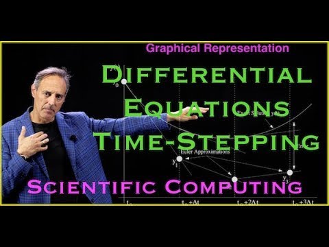
8:42 Now there's something more at play here which is this idea of stability that we're going to have to address. Okay. Now before we get into some of these details, let's just kind of graphically show what's going on here. The idea here is I start off with y not right that's my initial state of the solution. And how do I move to the future? Well, if you go back to that formula, it says that I go to the future by a slope formula, right? So here's the slope. So I take off on a tangent line, which is the slope, and I make a prediction about what the future state is, y1. Now this is the exact solution. Okay, so this is an exaggeration of how this would work.

9:25 But the idea is I'm making an approximation to the future state which is y1 when in fact I was supposed to be right here. But this is my step. I took a delta t step. And of course notice if I take smaller smaller delta t's you can imagine I stay much closer to that line. But this is a big step to exaggerate what's happened. So I'm at y1. This is my estimate for the future. Now I take this future point and I estimate the slope that would come from it from that value of y1 which is let's say this slope here that gets me to y 2. I now plug that back into f to get an estimate of the slope for y 2 and so forth. So notice that as I go forward in time I get what's called propagation of error.

10:11 I make a mistake going to the future of a certain size, but then I'm using that point to move to the next point to the future. So I not only do I make a mistake in that next step, it's compounded with the step I already made, the error I already made. I take another step. So I keep compounding error into the future. But the idea here is if I take delta t small enough, I could track this exact solution into the future. And right away we're going to have to start thinking about this from two different error metrics.

10:43 One is how much error do I do I make in just one step delta t. But ultimately I don't really care so much about that as if I make take many steps into the future. What's the error when I make an approximation to the future? And that's actually really the most important thing I want to do and is to sort of run this forward, roll it out, make a prediction from my dynamical system or differential equation. Roll it out there, see what it predicts. And I care about that prediction in the future, not just one delta t. Often one delta t is just not quite that interesting. So these are going to come in the in the names under the names of global and local error.

11:26 Global error is the thing we're really interested in. In other words, how much error do I accumulate over walking this forward in time and local error which is how much do I accumulate, you know, right in these next steps. So that's a graphical description and but we want to sort of back up a little bit because I'm already starting to show you in this graphical description some of the things that we got to think about which is I have to think about error. I have to think about cumulative error. I want to make sure I'm stable. In other words, when I walk that out, I don't want it to blow up. And so I want to think about this more broadly then in the time stepping scheme as time stepping maps. What I'm really looking at is the solution in the future is some function let's say of the current time.

12:11 Now actually there's different ways to think about this too. There are time stepping schemes usually the undergoing Adams bash forth Adams molton which can take multiple time steps in the past to approximate the future. So in other words, it wouldn't just rely on t of n. It rely on t of n minus one, t of n minus 2, and so forth with the idea that the more time points in the past gives me more accuracy in the future. That's how you'd want to use it. But for right now, let's just go with this scheme here, which is a one step. Here's where I am currently. I know my differential equation.

12:46 How do I take a step forward one delta t in time? Okay, so the approximation often revolves around this here. My solution in the future is what it is right now plus a little bit of something. So my point is I've got to compute what is that little bit of something I have to add to the current point to get to my future. So if delta t is small, the idea here is that if I take a future step and if delta t is small, the system shouldn't change too much. So whatever the state of the system is currently, all I have to do is give it a little bit of an update. So that's what this formula says. And the oiler formula gave us a very specific form of fee, but in fact, we can develop much more sophisticated algorithms to get much better accuracy and much better stability. Okay. So that remember we're always after that first and foremost accuracy and stability and finally if we can make it super fast as well we'll go for that as well. But baseline we have to make sure it's stable. We have to make sure it's accurate and then we can work on speed after those two are achieved.

14:00 So how do we actually start to evaluate schemes? How do we start to evaluate how to step forward and develop some more sophisticated schemes besides the oiler method? Well, it's going to come down to again tailaylor series expansions. This is always how we work this. This is how we make more accurate derivatives. This is how make more more accurate integration schemes. Always a tailaylor series expansion. So, what I'm going to do here is give you an estimate here of a tailaylor series expansion. What I'm going to say my future point, in fact, this is a generic representation.

14:33 what I'm going to do. Notice that when I walk into the future, I'm just using the current point. But as I walk forward, there's no nothing to stop me from using other points along the way. In other words, computing the derivatives along that future step. So what this is meant to represent is my solution in the future is what it is right now. the y of t plus delta t of I'm going to use here a which is some coefficient I know times the current value of f at time t plus b in other words a little bit I use a little bit of this estimate plus a little bit of this estimate but this estimate here notice what I'm going to do with this I'm going to evaluate the function f not at the current time but somewhere between the current time and the future time so P is usually between 0 and one. In other words, I'm going to go look out into the future and see what the derivative is doing. Where in the future? That's determined by P. I'm going to evaluate this function there and add these two together. So, in other words, I'm not just using the Remember, the Oiler scheme is all about just use the slope to go forward into the future, right? So, start from here. How do I get to the future? I take the slope and walk out. Well, what if I start I use some of that, but I also say, well, but in the future, the slope is kind of looking like this because I can actually estimate the slope in the future. And then I use those together to give me a better approximation of the future state. Okay? And that's what this formula is. So, I'm making this up. The things I don't know are the parameters here, A and B and P and Q.

16:11 But I can take this whole thing here and just tailor expand it all. Right? So again, I want to emphas I can't you can't I can't emphasize enough tailaylor series expansions are kind of like the entire heart of most of of numerical methods. Okay. So if you're good at tailor expanding, you could be successful in this field, right? And that's that's how we got most of our schemes. So we're going to tailor expand this and we're going to then make use of it. So let's look at this term here. So this is the term the second term right there. Okay, that we have in here which is this thing here evaluated halfway over and with some estimate for the next state of the solution. I can take that term alone and do a tailaylor series expansion right there with it.

16:58 Okay, so so far I haven't really done anything fancy except for I made up this form of solution which allows me to use the derivative estimate at the current point and somewhere in between now and the future and I tailor expanded this and now I can also just do a tailor expansion of this. Why have t plus delta t? Just do a tailor expansion of this term around t. Okay. So in other words, the left side, which is the future state, I tailor expand. The right side, which I made up this form, I also tailor expand. And guess what I'm going to do next? I'm going to match terms.

17:36 Okay? And when you match terms, you're going to get a system of equations. In fact, you're going to get three equations with four unknowns. And here's that they are. Remember, I just generically made up these parameters. A, B, P and Q. But here's what these parameters have to satisfy in order for my left tailor expansion to match the right tailor expansion. Okay, three equations, four unknowns. It means it's underdetermined, which means I can pick one of these parameters and by picking one of these parameters, all the other three then fall into place from there. This gives me the ability to create an infinite number of schemes.

18:20 right? Because it's underdetermined. So what we're going to do is look at some of the common ones. And some of the common ones, you pick the values of a. So a is 1/2 or a equals z. So a= 1/2 is what's called Jan's method. A is zero is called modified kosher oiler. And this is what you get when you pick those. So once you pick those, it allows you to determine b, p, and q because now you have three equations, three unknowns.

18:47 You plug those in and you now have these two new time stepping schemes. Okay? And so these are quite powerful because actually what they allow you to do is drop the error. The error in the oiler scheme was deltat t squared. And now by using a higher order tailor expansion you can drop the error further down. In fact that is the entire game in time stepping schemes. Remember, accuracy, stability. I can push accuracy down by using techniques like this with tailor expanding and tailor expanding terms so that I can get rid of terms, push the air out as high as possible.

19:28 That doesn't address yet the stability, but it addresses directly the accuracy. Okay? And what it basically is telling you is the more terms you use, okay? the more in the tailor expansion here you use you can kind of use those terms to push the error down. That's the idea. In fact, let me show you sort of what's sort of in some sense the most canonically used method sort of like this is your go-to method that you should I would always recommend using which is fourth order of brangakata.

20:02 Okay. So fourth order and a cuta has the following formula. How did we get this formula? A lot of tailor expanding. Okay. But the idea here is the solution in the future is what it is right now plus a little bit of a correction. Well, here's the correction. It comes in four stages. F1, which is the slope or f at the current point. So, use the slope at the current point to estimate the future plus 2 f_sub_2, which is basically computing the slope halfway out across you're taking a step delta t. So halfway across the domain, you do a slope calculation there based upon what you're predicting from here. Then you estimate f3 from f_sub_2. So in other I update my solution in the future. I produce another slope formula halfway across.

20:53 And then finally f4, which is estimate the slope at the terminus, which is the delta t across. And all of these numbers that you have here, including the values you have here, are determined by tailaylor series expansions which drop out terms and you push the error all the way to delta t to the 4th. So if I take a time step of 10us2, the accuracy is in fact in fact the error gets pushed out to 10 the minus5. The fourth here means it's 10 minus 4 globally. This is my cumulative error. The error over one step is 10 minus 5. So if I take a step of of 10 minus two, the error per step is 10 - 10. That's why you develop schemes like this. It's all about that accuracy. Okay? All about that action boss. It's a little Marawn from 2013.

21:49 Okay? And Marawn would love this. So, I don't know if he uses it, but you know, he probably would if he could. Look at that. He's got Seak green, green, blue. Okay, we're all good here. so there you go. That's the scheme. And the only thing else left for us to work with is this is how you do error. The only thing we have to think about now is stability. And stability is a very important issue, of course, with these time stepping schemes. But this one here, like I said, fourth order should be your go-to. You shouldn't use oiler. You shouldn't use other things. just use this. It's a great trade-off between accuracy and stability as a go-to method. Okay.

22:28 Now, first of all, before we use it though, we want to talk about how you have to set up all your differential equations because remember these are systems of first order equations that that is applied to. But look, I have a third order differential equation here. So, whenever you're given a differential equation, like for instance, this is a third order differential equation. your first job is to write it as a system of first order equations and then put it into Python as a system of first order equations.

22:59 So how do you do that? So first of all it's a third order equation. So if it's a third order equation because that's the highest derivative is three. What you're going to do is you're going to define a set of new variables. Let's call them y1 y2 y3 which is u first dative of u second d of u. These are going to be your new variables. You're going to trade out from working with u to y. Okay. And how do we do this transformation? Well, what we do is we differentiate each one of these. So y1 prime is u prime. y2 prime is second derivative of u. y3 prime is third derivative of u. And by doing that we can actually write down this first order system of equations. So the first one says y1 prime is y2. So y1 prime it's right here. So y1 prime is u prime but u prime is defined as u2 y2 right there.

23:54 This one here says y2 prime is equal to y3. So take the derivative of y2 prime. It's the second derivative of u which is y3. And then here is y3 prime. y3 prime is the third derivative of u. And by the way the third derivative of you is sitting right there. So there it is. So you take all those terms to the other side. You write them in terms of y1 and y2 and you have your differential equation specified. So you always have to do this step as the first thing once you're given a differential equation of whatever order you write it as a system of first order equations. There is the transformation of how to go from one to the other and that's how you do it.

24:37 Okay. So that sets us up for thinking about differential equations. what I really focused on this piece here was how to construct time stepping schemes. And remember for differential equations, it's really all about I want to take a step into the future. What is the most accurate way to do it? We haven't talked about stable way to do it, but the most accurate way everything's based upon a tailaylor series expansion and allows me to push the error down. But the ultimate thing that you have in time stepping is the solution in the future, one delta t in the future is what it is now plus a little bit of a correction. And so all these schemes are aiming at producing the best correction possible with the best error with the least amount of error possible. The only thing we have to think about now to make a stable scheme is how we're going to handle the stability idea. And so the next lecture is going to focus on that and then we'll implement some Vote.